Commercial Loan Calculator Methodology

Commercial loan calculators do one thing residential mortgage calculators do not: they size the maximum loan a property can support, not just the monthly payment on a loan you have already decided to take. That distinction is load-bearing. Everything else in CRE underwriting flows from it.

The sizing output is governed by three simultaneous tests, LTV, DSCR, and Debt Yield, and the lender extends whichever produces the lowest number. All three tests draw from the same upstream input. Which means a borrower who does not understand the framework cannot know which lever to pull, or why the number came back lower than expected.

Why NOI is the foundation every test is built on

Net Operating Income is what a property earns after operating expenses and before debt service. Simple enough. But the NOI figure a borrower submits and the NOI figure a lender actually underwrites are frequently not the same number, and that gap is where deals quietly lose proceeds.

Lenders are debt investors, not equity investors. That asymmetry is structurally significant, not a platitude. An equity investor cares primarily about upside: stabilization, rent growth, exit value. A lender cares about the downside case — think of it as the investor who checks whether the parachute works before admiring the view — specifically, whether cash flow holds up long enough to service the debt and preserve collateral value. That asymmetry produces systematic adjustments.

A lender will typically apply a higher vacancy and credit loss factor than the borrower's proforma reflects, because market conditions and tenant rollover risk are underestimated in optimistic projections. Reserves for replacement, often omitted from sponsor proformas, get deducted. Historical cash flows are weighted more heavily than forward projections. The lender builds a parallel underwriting model from the same rent roll the borrower submitted, and the two NOI figures can diverge materially before a single test has run.

Why does that matter structurally? Because NOI feeds all three tests. A conservative NOI adjustment does not tighten one constraint; it tightens all three simultaneously. A borrower who loses $50,000 in underwritten NOI does not just fail DSCR. The LTV-implied value drops, the Debt Yield ratio deteriorates, and the allowable loan falls on every axis at once. That compounding effect is underappreciated until you have watched it happen on a live deal — like pulling one thread and watching the whole sweater unravel.

How the LTV test converts property value into a loan ceiling

The formula is straightforward: Loan divided by Value, capped at the lender's maximum threshold. What is less obvious is that "Value" is not a number the lender accepts from the borrower. It is a number the lender derives.

The derivation works by dividing the lender's underwritten NOI by a market cap rate. A third-party appraisal eventually validates or adjusts that figure, but the lender's internal estimate sets the underwriting direction before the appraisal even arrives. This means two inputs drive the LTV ceiling: the NOI (already conservative, for the reasons discussed above) and the cap rate assumption. A higher cap rate produces a lower value, which produces a lower loan ceiling. The lender controls both.

Regulatory structure adds another layer. The OCC Comptroller's Handbook specifies supervisory LTV limits by asset class, and those thresholds function as hard ceilings in any compliant underwriting workflow. The High Volatility Commercial Real Estate designation under the standardized capital rules imposes a 150% risk weight, which creates a structural incentive to keep LTV within prescribed bounds regardless of what the collateral can otherwise support.

A typical institutional LTV constraint sits around 70%. The average CMBS LTV in 2024 was 54.9%. That gap is instructive. It reflects years of conservative sizing in which multiple constraints applied simultaneous downward pressure, not just the nominal LTV limit. LTV is, ultimately, a collateral test. It answers one question: how much of this asset's value are we willing to lend against? It does not ask whether the property can service the debt. That is a different test.

A deal constrained by LTV is generally a value problem. The path forward is appraisal support, a revised cap rate argument, or more equity.

How the DSCR test measures whether cash flow can service the debt

DSCR is NOI divided by annual debt service, with a minimum threshold that most lenders set at 1.25x. That ratio means the property generates 25% more cash flow than required to cover debt payments. The cushion is not decorative; it is the margin that absorbs income volatility before a loan moves toward distress.

What makes DSCR operationally more complex than LTV is that debt service is not a fixed input. It is produced by three interacting variables: the interest rate, the amortization period, and whether an interest-only period applies. Conventional commercial loan rates in 2025 and 2026 have ranged from roughly 6.5% to 9%, and a 100-basis-point move in rate changes the maximum loan that a given NOI can support in a meaningful and nonlinear way. A 30-year amortization produces lower annual debt service than a 25-year amortization, which means the same NOI supports a larger loan under the same DSCR constraint simply by extending the payoff schedule. Interest-only periods, by eliminating principal payments during the IO window, temporarily reduce annual debt service and allow a larger loan to pass DSCR during that period.

That last point is worth examining critically. Is IO a legitimate lever, or is it a structuring trick that inflates loan size without improving credit quality? The honest answer is: both, depending on context. For a value-add deal in lease-up, IO matches debt service to a period of below-stabilized cash flow, which is economically coherent. In a fully stabilized deal, IO primarily serves to maximize proceeds, and a sophisticated lender will scrutinize the refinance math at IO expiration accordingly.

DSCR is also the most rate-sensitive of the three tests. When rates rose sharply after 2022, deals that would previously have been LTV-constrained became DSCR-constrained, because the same NOI could no longer support the same loan at higher debt service costs. The binding constraint shifted across the market, not because properties changed, but because the rate environment moved.

A deal constrained by DSCR is a cash flow or rate problem. The lever is either NOI improvement, a more favorable amortization structure, or a lower note rate.

How the Debt Yield test removes rate and amortization from the equation

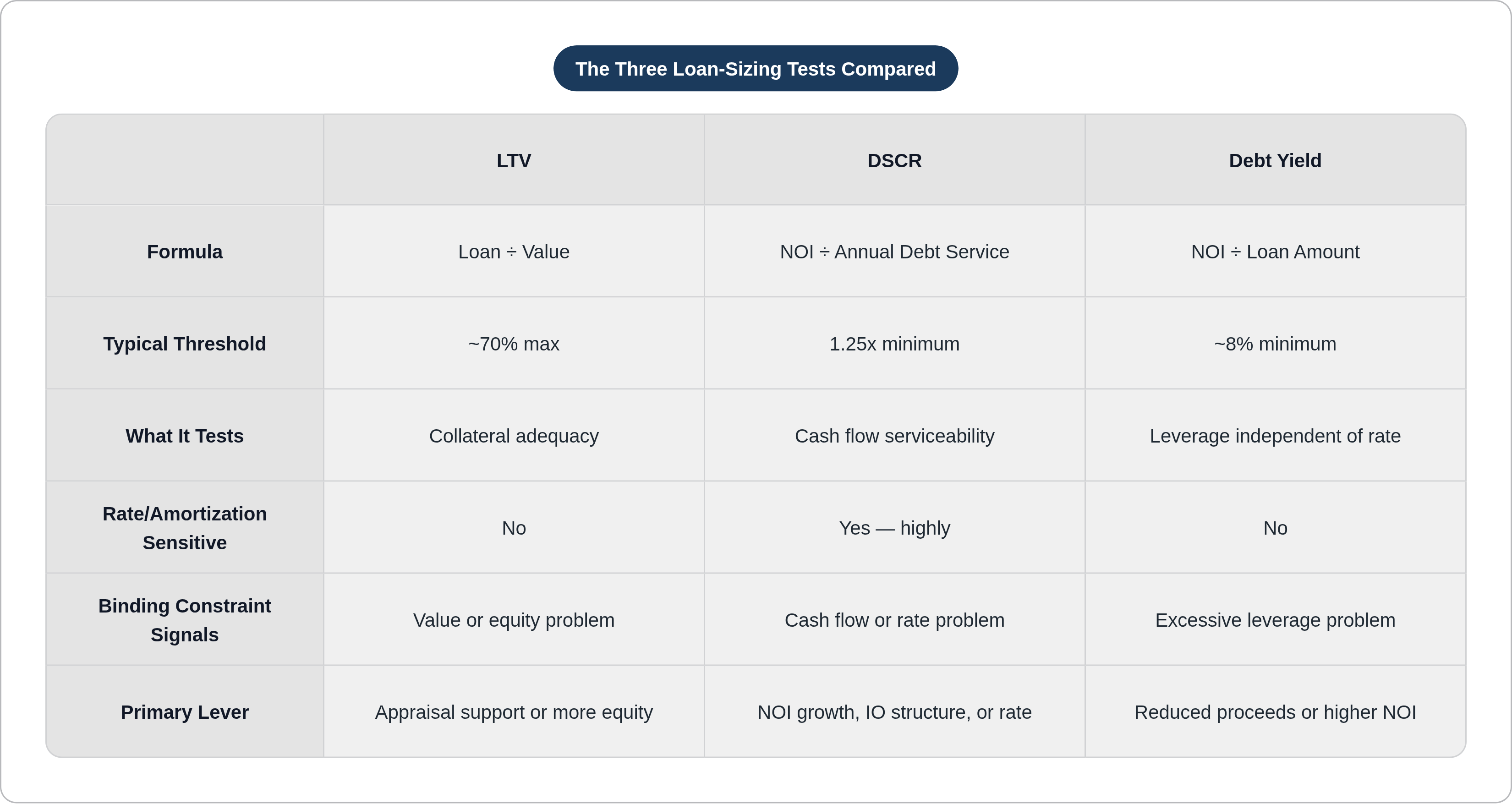
Debt Yield is NOI divided by the loan amount, expressed as a percentage. A typical minimum is 8%. What distinguishes it from DSCR is its indifference to rate and amortization: it is a direct, leverage-neutral measure of income relative to debt.

Why exactly does that matter? Because DSCR can be engineered. A lender willing to offer a low rate and a long amortization period can make a thin loan look adequately covered under DSCR while the underlying leverage remains excessive. Debt Yield closes that gap. For every $1 million lent, an 8% Debt Yield floor requires at least $80,000 of NOI, regardless of what the lender charges on the note. No rate assumption, no amortization schedule. The leverage itself must be defensible against income.

Lenders introduced Debt Yield largely in response to the low-rate environment of the 2010s, when generous amortization structures allowed thinly covered loans to pass DSCR screens. The metric became standard in CMBS and agency lending, where securitization introduces its own rate assumptions that differ from the originating lender's cost of funds, making a rate-independent measure of coverage especially valuable.

A deal constrained by Debt Yield is generally a leverage problem. The loan amount is simply too large relative to the property's income. The resolution is either more NOI before close or reduced proceeds.

The three tests now form a complete diagnostic picture. LTV addresses collateral adequacy. DSCR addresses cash flow serviceability. Debt Yield addresses leverage regardless of rate. Each test is designed to catch a different failure mode, which is why all three must run simultaneously.

Why the lowest result governs, and how to identify which test is binding

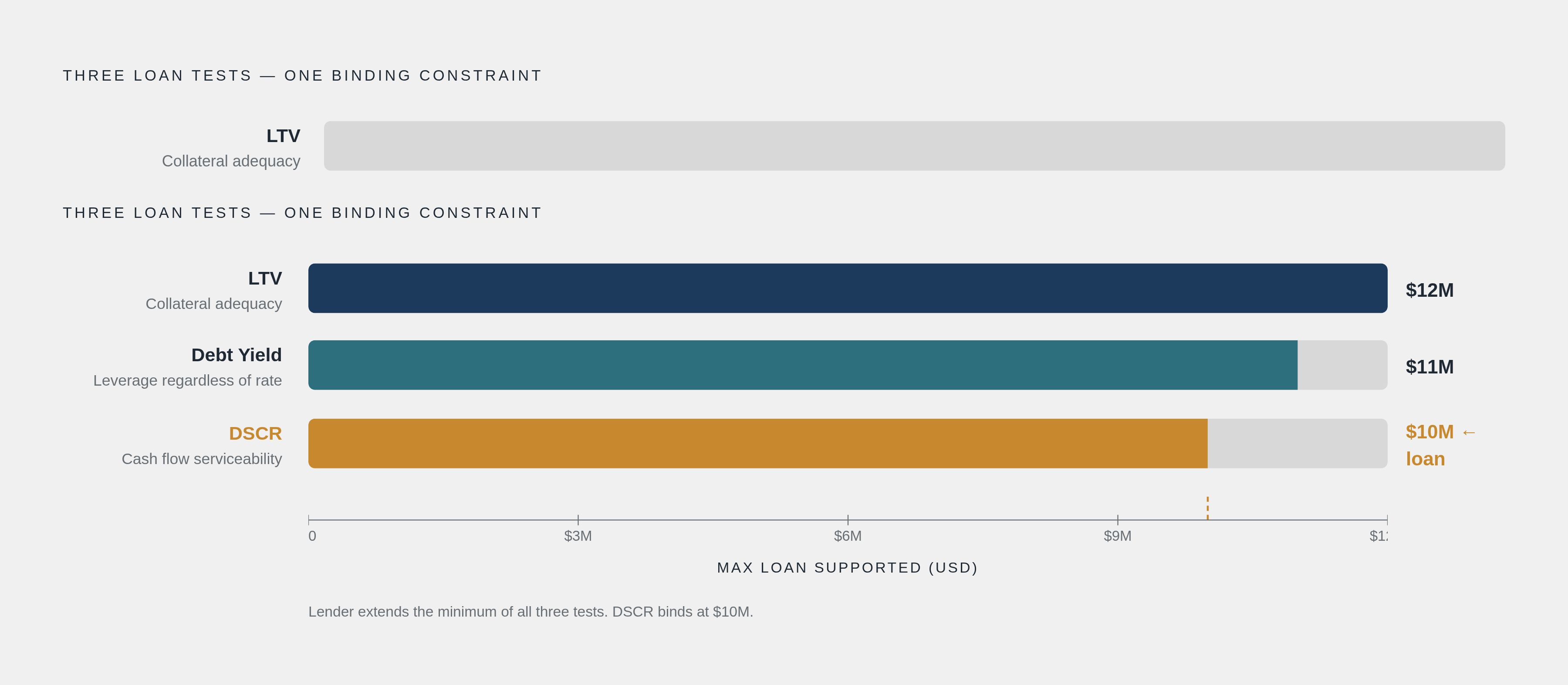
Each test produces an independent maximum loan amount. The lender extends the lowest of the three, because offering any larger loan would violate at least one constraint. The logic is not arbitrary conservatism; it is arithmetic. A loan that exceeds the DSCR ceiling is, by definition, a loan the property cannot service at the required coverage ratio.

Consider a worked example. If LTV supports $12 million, DSCR supports $10 million, and Debt Yield supports $11 million, the loan is $10 million. DSCR is the binding constraint. The borrower who argues for a better LTV appraisal has diagnosed the wrong problem — like fixing the roof when the foundation is cracked.

Identifying the binding constraint is the most actionable output of the three-test framework, because it tells the analyst exactly which variable to address. Binding LTV points to appraisal support or a cap rate argument or additional equity. Binding DSCR points to NOI growth, an IO structure, or a rate concession. Binding Debt Yield points to either reduced proceeds or higher income before closing. Misdiagnosing the binding constraint wastes time and negotiating capital on variables that are actually irrelevant to the deal.

It is also worth considering how the binding constraint shifts with market conditions. The post-2022 rate environment provides a clean illustration. Deals that were previously LTV-constrained became DSCR-constrained as debt service costs rose, even with property values and NOI relatively stable. The constraint migrated across the market without any individual property changing materially. A borrower or analyst running only one test at a time would have missed that shift entirely.

How break-even occupancy and stress testing extend the three-test output

Passing DSCR at stabilization tells you the property covers its debt today. Break-even occupancy tells you how far conditions can deteriorate before it stops doing so. A property with a 72% break-even occupancy has materially more cushion than one at 91%, even if both carry identical DSCR ratios at current occupancy. That distinction matters enormously in markets where demand volatility is a real credit risk.

Lenders calculate break-even occupancy to convert the DSCR ratio into an operational stress threshold. The two metrics move in tandem. A more conservative NOI assumption, with a higher vacancy load and reserves deducted, produces a lower DSCR and a lower break-even simultaneously. The lender's NOI adjustments compound through both metrics, which is why the normalization choices discussed in the first section are not academic.

Stress testing extends the analysis forward in time, particularly important given that most commercial loans carry balloon structures that force a refinance before full amortization. A lender underwrites not just whether today's DSCR passes, but whether the loan can be refinanced successfully at maturity. That requires running rate stress scenarios (what happens to DSCR if the refinance rate is 150 basis points higher?), occupancy stress scenarios (at what vacancy does NOI fall below debt service?), and exit cap rate scenarios (does the LTV constraint tighten at maturity if cap rates expand?).

The market-cycle relevance of disciplined stress testing is concrete. When credit conditions loosen, as they did during periods of historically low rates, the mechanical guardrails of stress testing become the primary structural check on underwriting quality. A lender who stress-tests consistently does not need market discipline to keep them honest; the methodology enforces it internally.

How loan type changes which tests apply and which inputs dominate

The framework described in the preceding sections is the base case: a stabilized acquisition or refinance underwritten on in-place NOI, with all three tests running on current cash flow. Most deals are more complicated than that.

Bridge loans are underwritten on two NOI scenarios simultaneously: current NOI, which is suppressed because the property is in lease-up or transition, and a proforma NOI reflecting the borrower's business plan at stabilization. Lenders often structure hold-backs that release additional proceeds as the business plan is executed and the proforma NOI materializes. The underwriting is dynamic in a way that stabilized analysis is not, and the credit judgment involves assessing the plausibility of the borrower's execution path, not just whether today's NOI covers today's debt service.

Construction loans are a different category entirely. The income-based tests largely do not apply during the construction period, because the property generates no income to underwrite. Instead, Loan-to-Cost and projected LTV on an as-complete basis govern the sizing. Interest reserves are built into the loan structure to cover debt service during construction. The binding constraints are cost underwriting and collateral projections, not DSCR or Debt Yield.

Prepayment structures introduce another variable. Yield maintenance calculates the present value of the lender's foregone interest, discounted at a reinvestment rate often benchmarked to a Treasury curve. When the note rate approaches or falls below the reinvestment rate, the penalty compresses toward zero; when the spread is wide, the exit cost can be substantial. Defeasance and step-down structures distribute that cost differently. A calculator configured only for stabilized analysis cannot accurately model these variations without explicit inputs for loan type and prepayment structure.

That is a category error, not a minor limitation. Bridge and construction deals have different binding constraints, different NOI inputs, and different risk profiles than stabilized assets. Using the wrong template produces not just an inaccurate number but an inaccurate characterization of where the credit risk actually resides.

Where manual calculation breaks down in practice and what follows

The three-test framework is conceptually elegant. Operationally, it is a grind.

Each test requires normalized NOI. Normalized NOI requires the analyst to reconstruct operating cash flow from borrower-submitted documents that arrive in inconsistent formats: operating statements organized differently by every property manager, rent rolls with varying line-item conventions, tax returns that require reconciliation to actual cash performance, and borrower schedules that do not align with any of the above. Before a single ratio can be calculated, an analyst has spent hours re-keying line items into a spreadsheet. CRE underwriting under manual workflows typically runs one to four weeks per deal, and the bulk of that time is consumed by document extraction and normalization, not by the credit analysis itself.

That raises an important question: is the bottleneck the methodology or the process? The methodology is sound. The bottleneck is the work that precedes it.

At portfolio scale, the problem compounds. Running the three tests across a maturing loan book to identify refinance risk or covenant stress requires the same normalization work, deal by deal, on a recurring basis. A lender monitoring fifty assets for DSCR covenant compliance cannot easily do that manually on a quarterly cycle without dedicating significant analyst capacity to mechanical work.

Purpose-built CRE underwriting platforms, including Hypha, address this by automating financial spreading, NOI normalization, and ratio calculation within the lender's own templates and underwriting conventions. The output, DSCR, LTV, and Debt Yield ratios grounded in the lender's own methodology, is produced in minutes rather than days. That compression matters not because speed is intrinsically virtuous, but because it reallocates analyst time from mechanical normalization to the credit judgment that the methodology is designed to support.

One argument holds that a capable general-purpose document tool achieves the same result. But the three-test methodology has CRE-specific conventions that a horizontal tool does not encode by default: lender NOI adjustment logic, cap rate derivation, balloon stress scenarios, loan-type-specific constraint hierarchies. A platform that treats a rent roll like any other structured document will extract the data without understanding what to do with it. The distinction is architectural, not a matter of marketing.

The framework this article has described, three simultaneous constraints, a single upstream input, a binding result that tells you exactly where to focus, is only as useful as the speed with which an analyst can apply it. When normalization is automated, the methodology becomes a starting point. When it is manual, it becomes the bottleneck, which is precisely the wrong place for the analytical work to stall.